Flux handling

Fluxes are a pain. The reason is that they require particular care to handle correctly.

Imports

Packages we’ll use in this notebook.

import matplotlib.pyplot as plt
import numpy as np
import scipy.interpolate

Example model

Let’s assume we’re solving the following simple energy balance model (although the model details really don’t matter too much for this discussion):

\[ C \frac{dT(t)}{dt} = F(t) - \lambda_0 T(t) \]

We want to solve the initial-value problem defined by this model combined with initial conditions. We want to solve for the temperature of the upper ocean (\(T\)) based on some input radiative forcing (\(F\)).

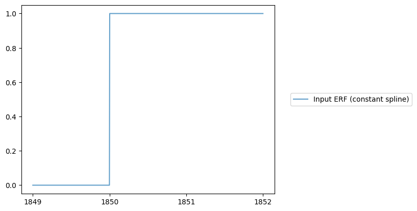
ERF

Let’s assume we are going to solve the model based on the following radiative forcing, with a constant interpolation between the discrete points when solving (for more on the different interpolation choices that can be applied to inputs, see Input interpolation).

erf = np.array([0, 1.0, 1.0, 1.0])
time = np.array([1849, 1850, 1851, 1852])
# We're using a constant interpolation,
# so we also calculate a continuous function
# that follows that assumption which we can use for plotting.
erf_constant_spline = scipy.interpolate.interp1d(time, erf, kind="previous")
# And a fine time axis for plotting
TIME_FINE = np.linspace(time[0], time[-1], 800)

# In a figure, it looks like this
ERF_PLT_KWARGS = dict(alpha=0.7, color="tab:blue", label="Input ERF (constant spline)")


fig, ax = plt.subplots()
ax.plot(TIME_FINE, erf_constant_spline(TIME_FINE), **ERF_PLT_KWARGS)

ax.set_xticks(time)
_ = ax.legend(loc="center left", bbox_to_anchor=(1.05, 0.5))

Temperature response

Just solving for the temperature is fairly trivial, this is just a standard initial-value problem. If we did this, we would get output something like the below.

constant_approx_tempreature_response = np.array([0.0, 0.0, 0.1, 0.16])

TEMPERATURE_PLT_KWARGS = dict(alpha=0.7, color="tab:red", label="Temperature response")

fig, ax = plt.subplots()
ax.scatter(time, constant_approx_tempreature_response, **TEMPERATURE_PLT_KWARGS)

ax.set_xticks(time)
_ = ax.legend(loc="center left", bbox_to_anchor=(1.05, 0.5))

Handling fluxes

The issue arises when we want to calculate the fluxes consistent with this model solution. For example, let’s say we want to calculate the net energy flux at the top of the atmosphere. This is given by:

\[ N = C \frac{dT(t)}{dt} = F(t) - \lambda_0 T(t) \]

From our temperature solution, we can trivially calculate the net energy flux at the points we have solved. If we did this, we get a solution something like the below (where the magnitude would depend on the size of the constants, so just focus on the shape).

constant_approx_instantaneous_n = np.array([0.0, 2.0, 1.6, 1.3])

N_SCATTER_KWARGS = dict(
    alpha=0.7, color="tab:green", label="Net energy flux discrete points"
)

fig, ax = plt.subplots()
ax.scatter(time, constant_approx_instantaneous_n, **N_SCATTER_KWARGS)

ax.set_xticks(time)
_ = ax.legend(loc="center left", bbox_to_anchor=(1.05, 0.5))

Integrating fluxes

However, let’s say we want to know what the cumulative heat uptake over the experiment is. To do this, we need to know what the flux looks like in between the reported discrete points. In other words, we need to work out how to go from the discrete points the solver has visited to a continuous function (a related problem to the one discussed in Input interpolation).

Assume behaviour between discrete points

We could simply make an assumption about this.

Constant spline

For example, we could use a constant spline (this is the same as assuming a left-hand sum in the integral).

n_constant_spline = scipy.interpolate.interp1d(
    time, constant_approx_instantaneous_n, kind="previous"
)

N_CONSTANT_PLT_KWARGS = dict(
    alpha=0.7, color=N_SCATTER_KWARGS["color"], label="Net energy flux constant spline"
)

fig, ax = plt.subplots()
ax.scatter(time, constant_approx_instantaneous_n, **N_SCATTER_KWARGS)
ax.plot(
    TIME_FINE, n_constant_spline(TIME_FINE), **{**N_CONSTANT_PLT_KWARGS, "alpha": 1}
)

ax.set_xticks(time)
_ = ax.legend(loc="center left", bbox_to_anchor=(1.05, 0.5))

If we did this, we are effectively assuming that the temperature is constant throughout the timestep. However, we know that it isn’t, it is dropping over time, so we would over-estimate the cumulative heat uptake (except in some special cases). So, this approximation clearly has some error.

Linear spline

Another option would be a linear spline (this is the same as using the trapezium rule in the integral).

n_linear_spline = scipy.interpolate.interp1d(
    time, constant_approx_instantaneous_n, kind="linear"
)

N_LINEAR_PLT_KWARGS = dict(
    alpha=0.7, color="tab:red", label="Net energy flux linear spline"
)

fig, ax = plt.subplots()
ax.scatter(time, constant_approx_instantaneous_n, **N_SCATTER_KWARGS)
ax.plot(TIME_FINE, n_constant_spline(TIME_FINE), **N_CONSTANT_PLT_KWARGS)
ax.plot(TIME_FINE, n_linear_spline(TIME_FINE), **{**N_LINEAR_PLT_KWARGS, "alpha": 1})

ax.set_xticks(time)
_ = ax.legend(loc="center left", bbox_to_anchor=(1.05, 0.5))

If we did this, we are effectively assuming that the temperature varies linearly throughout the timestep. This might be quite a good approximation in many cases. However, in this case, we know that it under-estimates the cumulative heat uptake because the analytical solution to this experiment is actually an exponential response. So, this approximation comes with some error too.

Having to approximate at all feels wrong. We have just solved the model, we should know the corresponding fluxes and cumulative fluxes at all solved points. It turns out that we do, we just have to tweak the way we solve the model slightly.

Error-free solution

The idea is that we include our cumulative fluxes as state variables of our model. In this instance, we might define our cumulative flux to be \(U\), such that

\[ \frac{dU(t)}{dt} = N(t) \]

Then, we can just include \(U\) in the state variables we solve for (with minimal effort because its rate of change of equation is trivial). This idea is discussed in much more detail in Ireson et al., GMD 2023, who also show that it is a performant way to handle this issue too. Thanks to @anorton for suggesting that we add this idea to fgen!

The nice thing about this solution is that it gives us values for cumulative flux that are consistent with the state variables we have solved for (almost by definition, because they are solved for at the same time and in the same way as the state variables). (We are pretty constant this is also true in the general case, but haven’t yet been able to prove it to ourselves given how many different combinations of model, inputs, interpolation schemes and solvers you have to think about). As a result, we end up with cumulative fluxes that don’t come with any approximation error, unlike the approaches discussed above (again, we’re pretty sure this is true, and we’re pretty sure the reason it works is that the cumulative fluxes are solved with the same set of steps [whether they be ‘full’ steps like in Euler forward solving approaches or combinations of steps like those used by Runge-Kutta fourth-order solvers] as the state-variables when it is done this way).

Going from the error-free cumulative fluxes back to fluxes

The method above gives us a way to calculate cumulative fluxes without error. However, now we need a way to go back to fluxes. This presents us with a different issue.

The problem is that cumulative fluxes and fluxes are related by integration/differentiation operations. These operations are only truly defined on continuous data. All operations which work with discrete data are implicitly making an assumption about how to convert from discrete to continuous data. For example, left-hand integration assumes a constant spline. Trapezium rule integration assumes a linear spline. Finite difference differentiation assumes a linear spline.

Key takeaway number 1

In order to ensure that the cumulative flux and flux data can consistently be converted from one to the other, you have to capture information about what sort of spline to use when converting them from discrete to continuous data.

The second problem is that, when you differentiate, you end up with one fewer time points in your timeseries than you started with. For example, if I differentiate the cumulative fluxes [0, 1, 3] with a time axis of [1850, 1851, 1852], assuming a linear spline, then I end up with [1, 2] on a time axis of [1850, 1851]. I don’t know what the flux is in the last step because I don’t have any information about the cumulative flux at the start of the last step, nor when that last step ends. (As a sidenote: as we assumed a linear spline for the cumulative flux, the consistent spline to use with the flux [that will reproduce the original cumulative flux if applied] is constant).

Key takeaway number 2

In order to ensure that the cumulative flux and flux data can consistently be converted from one to the other on the same time axis, you have to capture information about the time bounds. This ensures that you can differentiate and integrate with confidence about how long each time step is, particularly the last one.

Key takeaway number 3

In order to convert cumulative flux into flux with confidence, you need to have information about the cumulative flux at the start and end of the time step.

These takeaways are the reason that [TODO: once we’ve worked it out (for discussion, see #22), the rest of this notebook then discusses how we handle this issue].